Home

Beach morphology and its measurement

The beach is not a static surface: it continuously changes shape under the action of waves, currents, wind and storm events. Some areas accumulate sediment and advance towards the sea, others progressively lower until they disappear. Precisely measuring the sand elevation along a transect perpendicular to the shoreline, and repeating the measurement over time, allows reconstruction of the morphological history of the site and early identification of the areas most at risk of erosion.

The LiDAR system of the RVMC network automatically acquires the altimetric profile of the beach with a fixed laser scanner installed at height. From these scans, an automatic procedure calculates the mean profile elevation, quantifies cumulative variations with respect to the initial monitoring state and classifies each transect point based on its morphological behaviour over time.

Procedure overview

The process is structured in three sequential stages, executed in cascade on each set of acquisitions available for a station.

1. Preprocessing — each raw scan is geometrically corrected for residual sensor tilt, filtered for outliers and interpolated onto a regular spatial grid.

2. Multi-temporal analysis — the set of all processed scans is analysed to produce the mean profile, cumulative deviations with respect to the first acquisition and morphological classification into four behavioural types.

3. DGPS-RTK validation — periodically, ground elevation measurements acquired with high-precision DGPS-RTK instrumentation are compared with LiDAR profiles to verify the absolute accuracy of the system and, if necessary, calibrate the geometric parameters of the sensor.

The concept

Each time the laser sensor acquires a scan, the result is a point cloud: for each emitted ray, the system records the distance to the hit obstacle. Before different scans can be compared, it is necessary to “clean” these raw data: remove clearly erroneous points, correct small installation inaccuracies of the sensor and bring all profiles onto the same spatial grid.

This stage is comparable to sample preparation before a laboratory measurement: without it, the results of the subsequent analysis would be difficult to compare across different acquisitions.

Technical details

The preprocessor (lidar_analyzer.py) applies four operations in sequence to each raw sensor CSV file (columns: time, x, y, z, angle_deg, distance_cm):

1. Pitch correction — rigid rotation of the profile around the optical centre of the sensor to compensate for residual vertical tilt of the mounting bracket. The correction angle (θ_pitch) is determined for each station via linear regression on DGPS validation residuals (see Stage 3).

2. Adaptive outlier filter — based on the interquartile range (IQR) with configurable multiplier (default 0.5). The adaptive threshold is more tolerant in areas of low angular density (points far from the sensor) where natural dispersion is greater.

3. Regular grid interpolation — filtered points are reprojected onto the transect x_grid axis and resampled at a fixed step (default 0.5 m) via linear interpolation.

4. Diagnostic linear fit — estimation of the linear regression plane on the profile, useful for monitoring mean slope over time.

The geometric configuration of each station (sensor elevation, pitch angle, transect limits, sand threshold) is centralised in the lidar_config.yaml file.

Note on the optical centre of SICK LD-LRS sensors. In SICK LD-LRS sensors of the RVMC the optical centre (rotating mirror that emits the laser) results located approximately 14 cm below the mechanical fixing flange. Field measurements of sensor elevation refer to the mechanical flange and must be corrected with the appropriate offset (offset_y) to obtain the correct measurement geometry. Neglecting this correction introduces a constant systematic bias across the entire profile.

The concept

Once enough scans have been collected over time, the system compares them all together to understand how the beach has evolved. For each transect point it calculates two pieces of information: how much the elevation has changed since the start of monitoring (the cumulative change) and how unstable that point has been over time (the volatility). By combining these two measures, each profile point is classified into one of four categories.

Areas of steady accumulation show an increasing and stable elevation over time: sand is progressively deposited. Areas of irregular erosion are the most critical: elevation decreases over the medium term, but with large fluctuations that indicate an unstable system subject to recurring storm impacts.

Fig. 1 — Morphological volatility chart: each point represents a position along the transect. The horizontal axis measures the net cumulative change with respect to the first acquisition; the vertical axis shows volatility over time. The four quadrants identify the behavioural types TYPE 1–4.

Technical details

The multi-temporal processor (optimized_lidar_processor_v2_3_FIXED.py) loads the entire archive of interpolated profiles for a station and calculates, for each x_grid position:

• Temporal mean z̄(x) — mean elevation observed across all available acquisitions, produced in the file *_media_temporale.csv.

• Cumulative deviation Δz(x, t) = z(x, t) − z(x, t₀) — elevation change with respect to the first acquisition t₀, produced in the file *_deviazioni_cumulative.csv.

• Final cumulative value fc(x) = Δz(x, t_N) — net variation between the last and the first acquisition.

• Volatility σ(x) = std(Δz(x, t)) — standard deviation of cumulative deviations over time.

The combination of fc(x) and σ(x) determines the classification of each point:

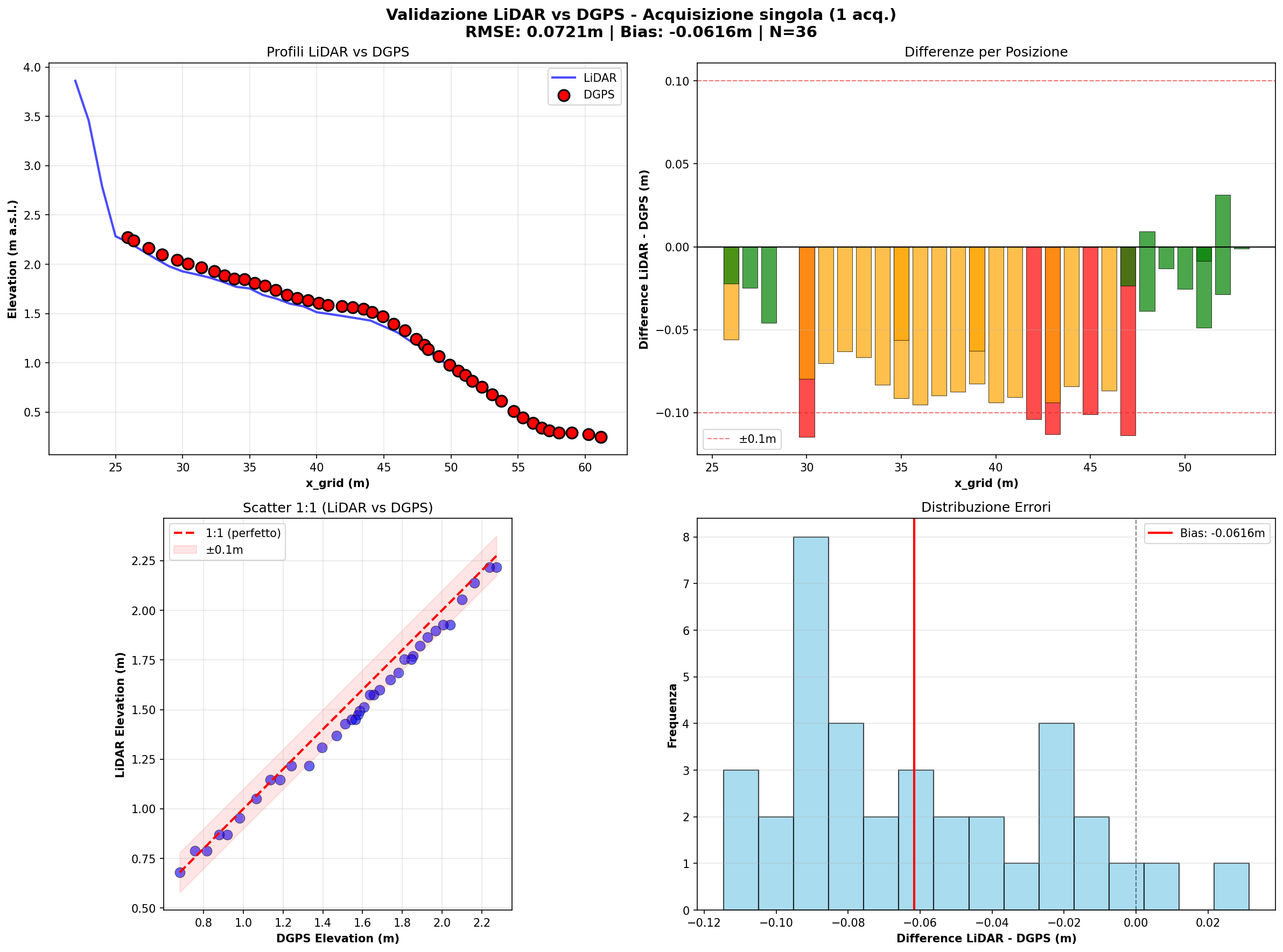
TYPE 4 identifies the most vulnerable sectors: environments subject to both net sediment loss and large fluctuations over time. It is the strongest response signal to erosion and accretion cycles induced by storm events. TYPE 4 points are highlighted with a red diamond symbol in the volatility chart.

The concept

To determine how reliable the LiDAR measurements are, periodically an operator physically walks the beach with a high-precision GPS receiver (DGPS-RTK), recording sand elevation at a series of points along the monitored transect. These field data, accurate to the centimetre, are then automatically compared with LiDAR profiles: the residual difference — the system error — is measured and, if necessary, used to correct the sensor geometry.

The process is similar to the periodic calibration of a measuring instrument: even a well-installed sensor can accumulate small errors over time, and comparison with independent measurements is the only way to detect and correct them.

Fig. 2 — Comparison between the LiDAR profile (solid line) and DGPS-RTK measurements (points). Agreement is evaluated via RMSE, systematic bias and spatial distribution of residuals.

Technical details

The validation script (validate_lidar_dgps_v2.py) takes as input the mean LiDAR profile of the station and a CSV file with field DGPS measurements (format: ID, East, North, H_geoid, UTM 33N, geoidal elevation). For each DGPS point:

1. Transect projection — the UTM position of the DGPS point is converted to x_grid coordinate along the transect axis via scalar product with the directional unit vector (azimuth configured per station).

2. Spatial matching — association with the nearest LiDAR point, within a configurable tolerance (default 0.5 m).

3. Residual calculation — LiDAR − DGPS elevation difference for each matched pair.

The calculated metrics are:

The operational quality levels defined for the RVMC system are:

When residuals show a systematic increasing trend with distance from the sensor (linear error in x_grid), the cause is a pitch error of the sensor rather than a simple vertical offset. In this case the script calculate_pitch_from_dgps.py estimates the corrective angle via linear regression:

residuo(x) = a · x + b   →   θ_pitch = arctan(a)

The estimated angle is entered in the station's lidar_config.yaml file and the entire pipeline is re-run from preprocessing. The planned validation frequency is every 6 months under normal conditions, and after any extraordinary event (sensor maintenance, severe storm, data anomalies).

Currently, two stations have been validated with field DGPS-RTK data. The results document the progression of the calibration process.

The Kufra station required a complete two-step calibration process: correction of the offset_y to account for the difference between mechanical centre and optical centre of the SICK sensor, followed by pitch correction of −0.61° estimated by linear regression on DGPS residuals (R² = 0.88, p < 10⁻⁷).

The remaining 3 LiDAR stations (Senigallia, Viareggio, Marina di Castagneto Carducci) are awaiting their respective field survey campaigns.

The network currently comprises 11 stations, of which 5 are equipped with SICK LD-LRS sensors, distributed along the Adriatic and Tyrrhenian coasts. Raw data are archived in CSV format on the ISPRA processing server and periodically processed through the pipeline described on this page. Results — mean profiles, cumulative variation maps and volatility charts — are available in the Multi-temporal LiDAR Analyser and in the LiDAR Scan Analyser.

The centralised configuration in lidar_config.yaml collects for each station the calibrated geometric parameters (sensor elevation, pitch angle, transect limits), DGPS validation status and the history of calibrations performed. The system is designed for future integration with the web portal videomonitoraggio.isprambiente.it via standardised JSON export.