Home

Wave runup and its measurement

The runup is the maximum uprush of water on the emerged beach during the swash cycle: the farthest point from the shoreline reached by the uprush wave front. Its position and elevation determine how much beach is flooded during a storm and how frequently. Monitoring runup over time allows assessment of beach exposure to meteo-marine events, estimation of flood risk, and calibration of numerical wave propagation models.

The RVMC network LiDAR system performs every day at 12:00 a continuous scan lasting 120 seconds, unlike the instantaneous scans at other times (06:00, 10:00, 14:00). During these 120 seconds the laser completes approximately 900 full rotations at 8 Hz, producing a dense time series of surface elevation — both of the emerged beach and of the water surface. From this series, the mean water level, its oscillations and the maximum runup position are automatically extracted.

Procedure overview

The process is structured in four phases, executed automatically every day on the 12:00 scan file.

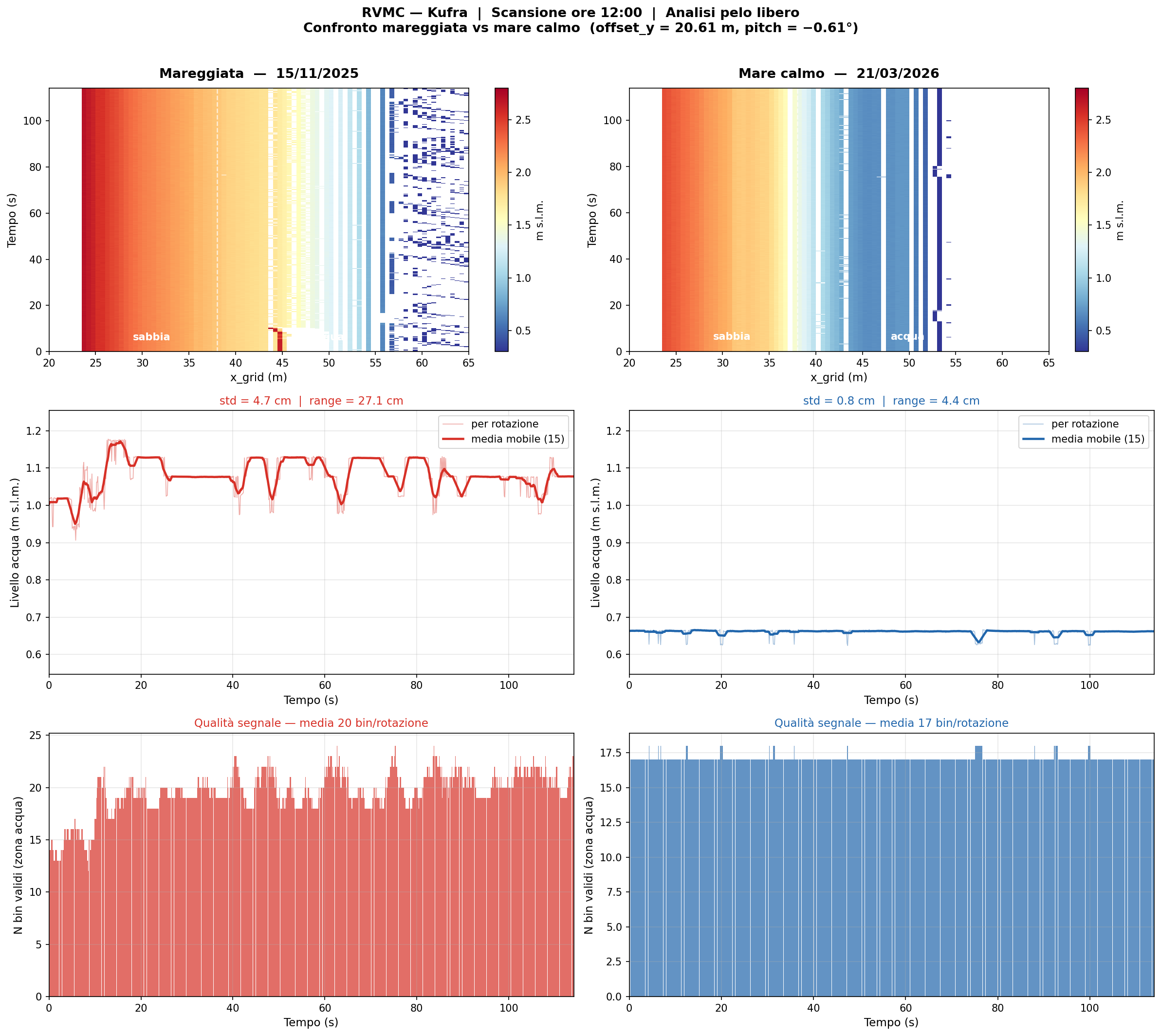
1. Rotation segmentation — the raw file is split into individual laser rotations (~550 points each, ~125 ms duration) by identifying the temporal gaps between consecutive rotations.

2. Heatmap construction — the ~900 rotations are organised into an elevation-time matrix: each cell contains the mean elevation measured in a 0.5 m spatial bin at a given instant. The heatmap displays the temporal evolution of the beach profile over the 120 seconds of acquisition.

3. Sand/water discrimination — an adaptive algorithm identifies the boundary between the emerged beach and the water zone by analysing the temporal variability of elevation in each spatial bin.

4. Metrics calculation — from the water surface time series, mean level, maximum level (runup), agitation index and horizontal beach inundation proxy are calculated.

The concept

The continuous measurement of a beach section provides, in our case, 900 measurements of ground elevation at each point along the transect. One way to represent, and therefore describe, the temporal trend of all these measurements e` fornito dall'immagine — heatmap — in cui l'asse orizzontale rappresenta la distanza dalla postazione del sensore, l'asse verticale il tempo, e il colore la quota del suolo o della superficie dell'acqua. Nella zona di spiaggia asciutta il colore è stabile nel tempo; nella zona dell'acqua il colore cambia ad ogni misura, riflettendo il moto ondoso.

Fig. 1 — Elevation-time heatmap for two meteo-marine conditions compared. Left: storm (15/11/2025), with strong chromatic variability in the water zone (x > 42 m). Right: calm sea (21/03/2026), with an almost uniform water zone that disappears beyond x = 53 m due to specular reflection.

Technical details

Individual rotations are identified in the raw CSV file by detecting temporal gaps greater than 50 ms between consecutive points (timestamps in microseconds). For each rotation and for each 0.5 m spatial bin along the x_grid axis, the mean elevation of the points contained in the bin is calculated, after applying the pitch correction and vertical offset calibrated for the station (parameters pitch_deg and offset_y in lidar_config.yaml). The result is a matrix (n_rotations × n_bins) with elevation in metres a.s.l., where cells without points are marked as NaN.

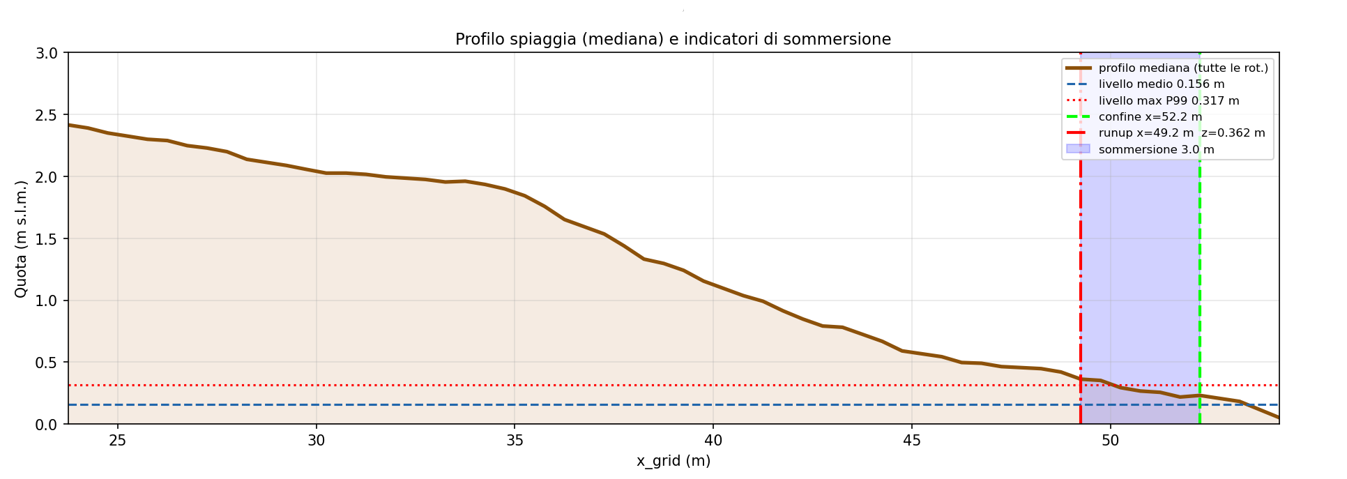
The reference beach profile is calculated as the median of all rotations for each spatial bin. The use of the median rather than the mean ensures robustness to temporary obstacles (people, objects) that may occupy the shoreline for some rotations producing anomalous elevations.

The concept

The dry beach is a rigid surface in the very short term: its elevation does not change between one laser rotation and the next. The water surface, on the contrary, moves with the waves: its elevation varies continuously over time. The system exploits this difference to automatically identify where the sand ends and the water begins — without needing to know the shoreline elevation in advance.

However, laser behaviour changes depending on sea conditions. With rough sea, the water returns a variable and recognisable signal. With calm sea, the water surface is nearly specular: the laser beam bounces away without returning to the sensor, producing not a variable signal but an absence of signal. This physical difference requires two distinct criteria to identify the sand/water boundary.

Technical details

For each spatial bin, two metrics are calculated from the heatmap:

• Temporal standard deviation std(x) — how much the elevation oscillates in that bin over the ~900 rotations. In dry sand std(x) ≈ 0.5 cm (instrumental noise); in rough water std(x) > 1.5 cm.

• Coverage cov(x) — percentage of rotations in which the bin receives a valid laser return. Sand has coverage ≈ 100%; specular water (calm sea) has coverage ≈ 0%.

The sand/water boundary is identified with a dual adaptive criterion, applied to the std(x) and cov(x) profile smoothed over a 2.5 m spatial window:

When both criteria are satisfied, the boundary closest to shore is chosen. The activated criterion is recorded in the output (criterion = A(std), B(no-signal) or A+B) and can be used as a qualitative indicator of sea state.

Note on wet sand and the saturation gradient. During storms, swash motion leaves a moisture gradient on the beach: zones closer to the runup limit are wetter than those further back. Wet sand behaves intermediately between dry sand and free water: laser reflection varies between one rotation and the next depending on the degree of saturation. This means that the boundary identified by high std represents not only the free water surface, but the entire active swash zone during the 120-second window. The boundary should be interpreted as an estimate of the swash influence limit, not as the instantaneous shoreline position.

The concept

Once the "water" zone is identified, the system extracts for each rotation the mean elevation of the water surface in that zone, building a water level time series with ~125 millisecond resolution. From this series, the mean level, oscillations and the point of maximum water uprush on the beach are calculated.

The mean level represents the water surface elevation independently of wave motion — it is influenced by tide and nearshore wave setup. The maximum level (99th percentile of the time series) represents the maximum uprush reached by the water in the 120 seconds of acquisition. The standard deviation of the level is the agitation index: low under calm conditions (approximately 0.5 cm), high during storms (typically 5–10 cm, with peaks above 20 cm).

Fig. 2 — Median beach profile (brown curve) with runup indicators. The dashed blue line indicates the mean water level; the dotted red line the maximum level (P99). The red vertical line indicates the x_grid position of maximum uprush (runup); the blue shaded area shows the beach reached by the water.

Technical details

The metrics calculated for each acquisition are as follows:

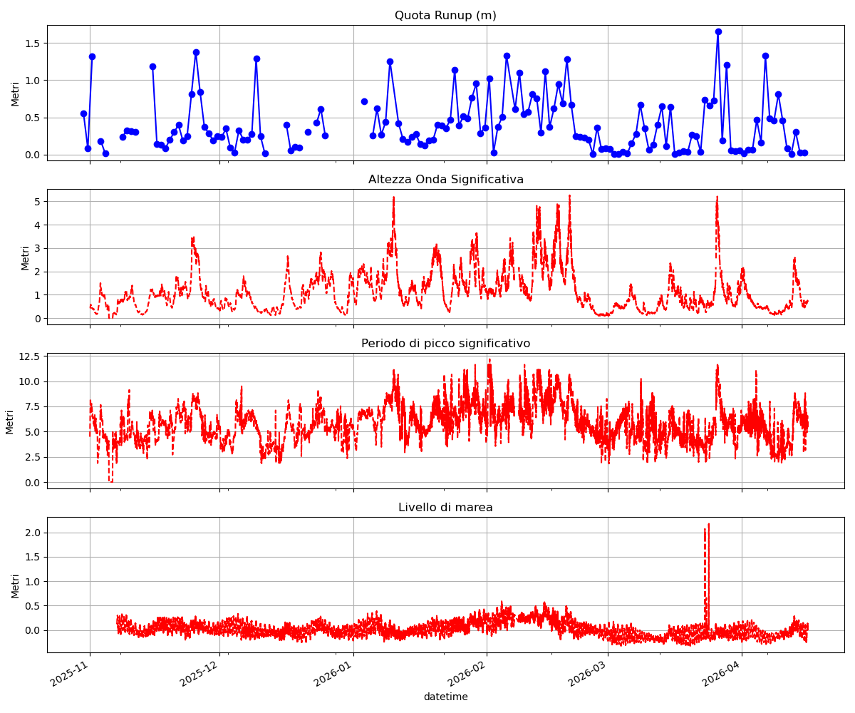
When the surface is specular (calm sea, criterion B), rotations beyond the boundary return no signal and the level cannot be measured directly. In this case the level is estimated from the elevation of the median profile at the boundary position (last point with laser return), and the speculare column in the output CSV is set to True.

The concept

The metrics calculated every day are archived in a time series that accumulates over time, allowing reconstruction of the runup history and sea state for each network station. The following chart shows how runup varies over the months, with peaks corresponding to winter storms and low values during fair weather periods.

Comparison with offshore wave data (significant wave height, peak period) and tide level allows contextualisation of each event and verification of the physical consistency of results.

Fig. 3 — Time series of runup elevation (upper panel) compared with significant wave height H_s, peak period T_p and tide level measured offshore of Kufra station (November 2025 – April 2026). Runup peaks coincide with the most intense storm events.

Technical details

The operational procedure is executed automatically every night at 05:00 by the ISPRA processing server (ecap1). The script analyze_water_level.py processes the 12:00 file for each station and appends a row to the historical CSV file ({stazione}_runup_timeseries.csv), first checking that the date is not already present to avoid duplicates. At the end of processing, the JSON for the web portal ({stazione}_runup_timeseries.json) is regenerated with updated data in parallel arrays format, directly compatible with Chart.js for client-side visualisation.

Data arrive on ecap1 the previous night via automatic FTP download (03:00 cron), making the previous day's data available on the portal with a maximum delay of approximately 26 hours from acquisition.

03:00 — CSV download via FTP from all stations
04:00 — file list generation for the portal
05:00 — runup analysis + portal JSON update

The LiDAR system and the MOVICO system operate in parallel on the same stations and complement each other in runup analysis. MOVICO extracts the planimetric shoreline position in UTM coordinates from timex images, providing the horizontal component of the uprush (where the water reaches in plan). The LiDAR measures the absolute elevation of the surface, providing the vertical component (at what elevation the water arrives).

The combination of the two measurements underpins the estimation of foreshore slope:

tan(β) = Δh / Δx

where Δh is the elevation difference between two shoreline positions corresponding to different water levels (derivable from tide gauge data), and Δx is the planimetric displacement measured by MOVICO. Foreshore slope is a fundamental parameter for assessment of coastal flood risk and for the empirical estimation of runup using the Stockdon et al. (2006) formulations.

Main methodological references:

• - Stockdon et al. (2006) — Empirical parameterization of setup, swash, and runup. Coastal Engineering, 53(7), 573–588.
• - Vousdoukas et al. (2012) — Reflective beaches and runup characteristics during storm conditions. Journal of Geophysical Research, 117, C09025.
• - Holman & Guza (1984) — Measuring run-up on a natural beach. Coastal Engineering, 8(2), 129–140.
• - SICK AG (2021) — LD-LRS Operating Instructions. SICK Sensor Intelligence.