Home

Shoreline monitoring

The shoreline represents the instantaneous boundary between the beach and the sea. Its position varies over time under the effect of tides, wave motion and long-term erosional or depositional processes. Systematically monitoring this position allows detection of beach retreat or advance trends, assessment of the effect of extreme meteo-marine events and support for integrated coastal management.

The MOVICO system (Coastal Video Monitoring) continuously acquires images from RVMC video monitoring stations distributed along the Italian coasts. From these images, an automatic procedure extracts the shoreline position on an hourly basis, produces time series and converts measurements into real geographic coordinates, making the data immediately comparable with field measurements and integrable into GIS systems.

Extraction procedure overview

The process is structured in four phases: a preparatory model-building phase (executed once) and three operational phases executed in sequence on each available image.

0. Dataset construction and training — manual selection and annotation of historical images stratified by sea state; training of the segmentation model on GPU.

1. Semantic segmentation — the deep learning model classifies each image pixel as water or non-water, producing a binary mask.

2. Shoreline extraction — the mask contour is geometrically analysed to isolate the relevant shoreline segment and measure its position along predefined transects.

3. Georeferencing — pixel coordinates are converted into metric UTM coordinates via back-projection with elevation constraint, using camera optical calibration and ground control points (GCP).

The concept

Before images can be analysed automatically, the system must be “trained”: a set of images is selected and manually annotated by experts, who precisely trace the boundary between water and sand. These images constitute the reference dataset from which the model learns to recognise the shoreline autonomously.

To ensure the model performs well under all meteo-marine conditions, images were selected in a balanced way: a similar proportion comes from days with calm, moderate, rough and stormy sea. This strategy — called stratified sampling — prevents the model from learning to recognise the shoreline only in the most frequent conditions, which would make it inaccurate during storms.

Technical details

Images were selected from the MOVICO historical archive using the script select_training_images_wavebuoy.py, which stratifies by sea state according to the simplified Douglas scale, using the significant wave height H_s from the CMEMS wave model (wavebuoy):

Annotations were produced with the CVAT tool (Computer Vision Annotation Tool), drawing binary water/non-water masks in polygon and RLE format on 543 images from 7 stations of the RVMC network: TorreCerrano01, acciaroli01, battipaglia01, fogliano01, kufra, senigallia, torresole01.

The dataset was split into training and validation with a station-stratified split (80/20, seed=42), ensuring each station is represented in both sets:

The 10 unused images were annotated in CVAT but the corresponding image file was not available on disk at the time of training. Actual split: 429 training images / 104 validation images.

The concept

The camera acquires every hour a timex image (15-minute temporal average of video), which attenuates wave motion and stably reveals the swash zone. An artificial intelligence algorithm automatically analyses this image and identifies the area occupied by water, distinguishing it from dry sand and other scene elements (structures, vegetation, sky).

The result is a binary mask: each point of the image is classified as water or non-water. The boundary between the two areas corresponds to the shoreline.

Fig. 1 — Timex image with the automatically extracted shoreline overlaid (red line). The timex is a 10-minute average of video acquisition that attenuates wave motion.

Technical details

The model used is SegFormer-B1, un'architettura transformer per la segmentazione semantica di immagini, eseguita tramite runtime ONNX on CPU for maximum portability and inference speed. The model was trained on a dataset of 533 immagini annotate manualmente from 7 RVMC network stations, with binary water/non-water masks produced with the CVAT annotation software.

Preprocessing faithfully replicates training conditions: resizing to 512×512 pixels, ImageNet normalisation (mean=[0.485, 0.456, 0.406], std=[0.229, 0.224, 0.225]), reconversion to original resolution with nearest-neighbor interpolation for the mask.

Validation set metrics (104 images, 7 stations):

The validation set mIoU (0.9743) is slightly higher than the training value (0.9737), indicating absence of overfitting and excellent generalisation capacity. The median boundary error of 0.2 pixels is consistent with the precision of manual annotations, indicating that the model has learned classification patterns consistent with human annotators.

The concept

Once the water/non-water mask is obtained, the system automatically identifies the contour of the wet zone and measures where the shoreline intersects predefined segments — called transects — that start from the dry beach and point towards the sea. Position is expressed as pixel distance from the transect starting point (landward side), and updated every hour to build the shoreline position time series.

Each camera can have up to 10 independently configured transects, allowing monitoring of different sectors of the framed beach.

Technical details

The binary mask contour is extracted with cv2.findContours and geometrically filtered via the "elbow" algorithm (maximum local curvature along the contour profile): this step separates the actual shoreline segment from the horizon line, which would also appear as a water/sky boundary in cameras with lateral geometry. The final selection criterion favours the longest segment among the candidates.

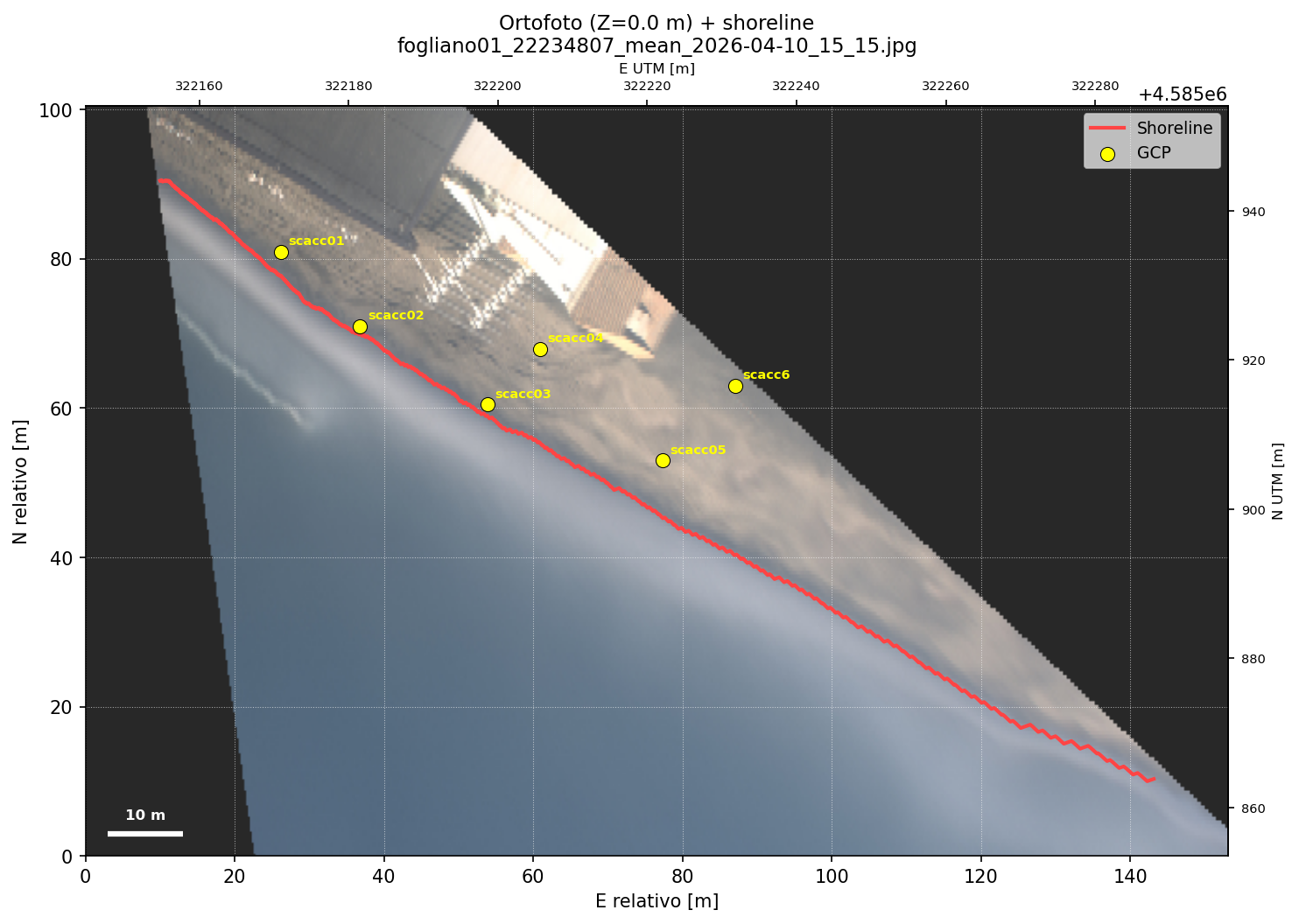
Transects are defined for each camera in YAML configuration files, with convention P1 = landward side, P2 = seaward side. The intersection between the contour and each transect is sampled with 1000 equidistant points. The result is archived in CSV format with columns timestamp, image, T01_dist, T01_status, T02_dist, T02_status, ... for each active transect.

The operational success rate is approximately 85% (17 out of 20 active cameras). The main skip reasons are: missing timex file (~10%) and failure of the elbow algorithm under extreme meteo-marine conditions (~5%).

The concept

Pixel positions are useful for relative monitoring (has the beach widened or narrowed?), ma per confrontare i dati con misurazioni di campo, rilievi LiDAR o immagini satellitari occorre esprimere la posizione in coordinate geografiche reali. This is the objective of the georeferencing phase: each shoreline point is converted to metric coordinates in the UTM reference system, directly integrable into GIS.

The conversion is based on camera geometry, known through a calibration procedure that uses ground control points (GCP): physical points clearly identifiable in the image whose precise GPS coordinates are known.

Fig. 2 — Georeferenced shoreline represented in UTM coordinates (plan view). The ground control points (GCP) used for calibration are indicated.

Technical details

The method is depth-constrained back-projection (DLT). Given the camera pose — rotation matrix R and translation vector t, ricavati con cv2.solvePnP dai GCP — and the beach plane elevation Z_const, per for each pixel (u, v) the system is solved:

s · [u, v, 1]^T = K · (R · [X, Y, Z]^T + t)
→ X, Y = f(u, v, Z_const, R, t, K)

The pixel_to_world() function is numpy-vectorised and operates on all N contour points with a single matrix multiplication (3×N), approximately 150 times faster than an equivalent Python loop.

The metric distance from transect point P1 is calculated as projection along the transect axis (not direct Euclidean distance), more robust in the presence of small lateral offsets. UTM coordinates of P1 and P2 are calculated once per transect and cached.

Optimal GCP selection occurs automatically: among all combinations of 6 points extracted from the available set, the system chooses the combination that minimises the reprojection error and saves it for subsequent runs. The typical reprojection error is less than 1 pixel.

Outputs produced for each image:

The pipeline is running on the ISPRA elaboration server (called ecap2). Un automated process (cron job) activates every hour, downloads the latest timex image available from each of the ~20 active cameras, executes the entire sequence segmenting → extraction → georeferecing and archive results on the server where is running the RVMC web portal (called ecap1).

Processing time per camera is approximately 1-2 seconds (ONNX inference + extraction), making the system suitable for hourly updates on standard hardware without dedicated GPU. Shoreline position data are available on individual station pages and in the Shoreline position section.

Main methodological references:

• - Xie et al. (2021) — SegFormer: Simple and Efficient Design for Semantic Segmentation with Transformers. NeurIPS 2021.
• - Holman & Stanley (2007) — The history and technical capabilities of Argus. Coastal Engineering, 54(6-7), 477–491.
• - Boak & Turner (2005) — Shoreline Definition and Detection: A Review. Journal of Coastal Research, 21(4), 688–703.